Setting Initial Conditions

<previous: Boundary Conditions	up to Table of Contents	next: Solution Options >
open Reference Guide (in this window) open Applet Page (in new window)

Setting Initial Conditions

    The initial conditions are the next step in setting up a problem, and can be found on the same navigation tab as the boundary conditions (see Fig. 11). At the bottom of the pane, below the left and right boundary panels are the options for setting initial conditions. Picking good initial conditions for a steady problem controls the progress of the solution. Good initial conditions will converge quickly, while poor initial conditions will converge slowly or not at all. For transient problems, initial conditions will be an intricate part of the problem definition. There are five choices for setting initial conditions: (1) setting from the left boundary condition, (2) setting from the right boundary condition, (3) setting constant, uniform initial conditions, (4) setting pointwise initial conditions, and (5) setting pointwise initial conditions from a file.
    The first two options, initializing from the left or right boundary are available only if that respective boundary has been declared as an inlet. If not, then this choice is grayed out. If the boundary is an inlet, Gryphon will apply the inlet boundary condition values to every single cell in the domain uniformly. This forms the initial condition of the problem. This choice is probably the most common, and is a good default choice for most steady state problems. With either the left or right boundary condition selected, the initial conditions are not applied until the user actually starts the solution. This is done in case the user changes the boundary values at the last minute, so that the solver will have the most up to date initial conditions available. This practice can be overridden by pressing the "conditions" button next to the radio selections. Gryphon will apply the currently defined boundary immediately to the solution. If there is an existing solution on the grid, Gryphon notifies the user that the new initial conditions will have no effect until the exisiting solution is completely deleted or the solution is started fresh again.
    The third option is to initialize the domain uniformly with values just as described above, but with user specified values which do not correspond to the boundary conditions. This is often useful if initializing from the boundary conditions has previously produced a divergent solution or poorly converged results. This can occasionally happen. In this case, those conditions need to be typed in. Pressing the "conditions" button now brings up a dialog box shown in Fig. 14.

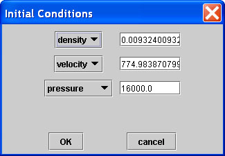
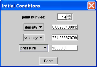
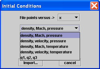
Figure 14. Uniform Initial Conditions Dialog Box

This simple box allows three parameters to be entered. First, density must always be known. Then, the user has a choice between velocity or Mach number. Finally, temperature or pressure must be specified. Pressing "OK" will set the conditions.
The fourth option allows more complex control. Pointwise initialization is most useful for setting up transient problems, but may be necessary to initialize a highly sensitive steady flow. Figure 15 shows the dialog box that appears when the "conditions" button is pressed here.

Figure 15. Pointwise Initial Conditions Dialog Box

The same choices are presented to the user here for properties to specify -- i.e. density, either mach or velocity, and either temperature or pressure. However, above these areas, the user can use the point number spinner to index cell by cell and change individual values for only that cell. The values are updated each time the spinner is changed to a new point number and when the user presses "Done."
Finally, the user can elect to import initial condition data from a file. Pressing the "conditions" button will bring up a dialog box as shown in Fig. 16.

Figure 16. Initialization by File Dialog Box

Like similar points in Gryphon, an ASCII text file is required which must be a total of four columns of data. The first column can be either an x position or a cell number like in the pointwise initialization above. Initial conditions versus spatial coordinate are most common. Then, the remaining three colummns must be one of the five possible forms shown, and they must be in the given order for proper interpretation. Here, the various combinations of properties seen before are available, along with the option to import the three conservative variables directly. This option might be useful if an earlier solution from some other program was available. Making the relevant selection and pressing the "Import..." button brings up a standard system file open dialog to select the text file. The file import option is most useful for time dependent problems like shocktubes. In cases such as that, one wishes to put a constant initial condition on one half of the problem domain and another constant initial condition on the remaining half. Instead of typing in the initial conditions point-by-point, they can be set by creating a 4 line initial condition file.

<previous: Boundary Conditions

up to Table of Contents

next: Solution Options >