Setting and Managing Boundary Conditions in Gryphon

<previous: Generating a Grid	up to Table of Contents	next: Initial Conditions >
open Reference Guide (in this window) open Applet Page (in new window)

Setting and Managing Boundary Conditions

    In general CFD analysis, boundary conditions are often the most complex part of the code. In one dimension, the boundaries consist of only two points, yet even in Gryphon they are an involved aspect of the code. Boundary conditions are what drive the problem, so it is important to correctly represent them.
    In any CFD calculation, there are two general classes of boundary conditions -- steady and transient. A steady boundary condition is obviously one which does not change with time as the calculation is run. A transient condition will change with time. In an overall steady-state CFD calculation, the boundary conditions must also be steady. In a transient calculation, a boundary condition can be transient or it could be steady (and something else could be time dependent in the problem). Gryphon automatically makes an analysis transient when a transient boundary condition is selected.
    Regardless of steady-state or transient, there are four types of boundaries implemented in Gryphon:

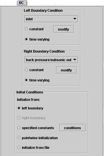
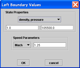
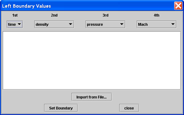
inlet - In an inlet, all conditions are known and applied from the exterior. The user must specify a speed, but this can be either velocity or Mach number. In addition two properties are required to completely define the thermodynamic state of the inlet. Valid combinations can be any one of the following: pressure and temperature, density and pressure, density and temperature, density and stagnation pressure, or density and stagnation temperature. If the flow is supersonic, the inlet condition completely defines the flux at the boundary. If subsonic, one characteristic is generated from the interior of the domain.
back pressure - A back pressure condition is an outlet condition which specifies only the pressure on the outlet and gets all other information from the interior. Pressure, and only pressure, must be applied. This condition is most often used for subsonic outlets of nozzles and pipes.
wall - The wall is a condition in which velocity is forced to zero on the wall and all other conditions are taken from the interior. The wall is typically used in shocktube problems, and is most likely used in transient calculations where characterisitic waves can reflect off the wall. No user input is required or allowed for the wall condition -- velocity is automatically set to zero.
extrapolation - The extrapolation condition is most useful for supersonic outlets for nozzles and similar problems. Extrapolation gets all information fro mthe interior, and results in effectively setting the first derivative of all variables to zero at the outlet. This condition causes some local disruption right at the outlet, but is an appropriate condition for many supersonic applications.

These four boundary conditions are set using the second of the navigation tabs -- the Boundary Condition tab. This is shown in Fig. 11. Boundary conditions can be applied either before or after the grid has been generated, but it makes the most sense to do it afterward.

Figure 11. Detailed View of the BC Navigation Tab

With the boundary condition tab open, the left boundary and the right boundary are visible. The type of each boundary from the list above can be selected via the choice box in each boundary section. The user can also pick if the boundary is to be steady or transient with the click of a radio button. A wall or extrapolation boundary condition requires nothing more. The mechanics are handled internally by Gryphon. A back pressure or an inlet condition however requires additional input from the user to specify the necessary properties. This input comes from pressing the "modify" button in each boundary panel.
For steady boundaries, a dialog like the one shown in Fig. 12 appears. For an inlet, the user simply picks the choice of state properties and speed parameters from the choice boxes and enters the respective values in the text areas. Properties should be entered in the boxes in the order that they are listed in the choice box just above. This is the same for specifying a back pressure condition, except that pressure will be the only available choice, and only the first text box is not grayed out.

Figure 12. Steady State Boundary Condition Specification Dialog

For transient flows, the boundary conditions must be entered as a function of time. Opening a dialog for a transient inlet will show a dialog box like the one in Fig. 13. Here, Gryphon expects a list of four columns of data, separates by spaces or tabs much like the grid importing algorithm discussed earlier. The user has a choice of which column contain which set of values in the choice boxes above the text area. The choices should be set as the columns of data are organized left to right. In the text area, the user has two choices. Data can be typed in by hand in the appropriate format, or data can be read in from a text file by pressing the "Import from file..." button just below. This imports a data file into the text window containing the entire contents of the file. At this point the contents can be manipulated before the boundary is read. In order to set the boundary, the user MUST PRESS the "Set Boundary" button at the bottom. Pressing close will simply close the dialog without saving changes. Press close only after the boundary has been set satisfactorily.

Figure 13. Transient Boundary Condition Specification Dialog

The back pressure condition works exactly the same way as the inlet except that only two columns of data are required and pressure is the only choice in the dialog boxes. Setting the boundary works the same.
Since the transient boundary data is discrete, and running a transient analysis with a specified CFL condition is likely to mean that timesteps will fall in between the available boundary data points, Gryphon once again linearly interpolates between adjacent points to get the effective boundary condition at a given timestep. Also, it is important to note that the boundary data is automatically assumed to be periodic in time. Thus, for example, if one second worth of data is input into the window and a calculation is run for 2 seconds, the second half of the calculation will apply the same set of data over agin that was used for the first second. This process repeats infinitely.

<previous: Generating a Grid

up to Table of Contents

next: Initial Conditions >