<previous: Solution Options
up to Table of Contents
next: Solution Control >
open Reference Guide (in this window)
open Applet Page (in new window)

Graphing Options

    Grpyhon supports powerful graphing options.  The visualization of the solution data is done thorugh the use and control of two separate windows.  As shown in Fig. 1, there is a line graphing window panel, and a geometry and contour graphing window panel.  Either or both of these capabilities may be used.  Figure 18 shows a detailed view of the graphing navigation panel, illustrating the various control options for the graphs.  It is important to first note that any changes made to the graph navigation panel will not take effect until the "Update Graph" button is pressed at the bottom.

Graphing Navigation Tab  
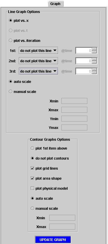
Figure 18. Detailed View of Graph Navigation Panel

    First, controlling the line graph will be discussed.  The line graph offers 3 choices of plotting types, some or all of which may be available depending on the problem type.  Until the grid has been initialized with a solution, the line graph will not respond and remains blank.  Once a solution has been generated by pressing "Solve" or at least initializing from the initial conditions, the user can select from plotting versus spatial coordinate, versus time value, or versus iteration number.  This choice may be made by selecting the appropriate radio button near the top of the line graph subpanel.
    When the user wants to plot something versus spatial coordinate (x) or versus time (t), the three choice boxes just below the radio buttons become active.  The user is offered the various choices listed in Table 1.  The line graph can display, 1, 2, or 3 lines simultaneously as indicated by the "1st","2nd", and "3rd" prefixes to the left of the choice boxes.  Selecting the first option "do not plot this line" obviously does not plot that available line on the graph.  Make any other choice plots the selected quantity.  Any quantity of interest is given in the choice menu.  If the solution is a steady state solution, the user cannot select to plot versus time (since there is no possibility to do so).

Table 1. Spatial and Temporal Domain Graphing Options in Gryphon (available for each line)
0
no line
1
pressure
2
temperature
3
density
4
velocity
5
Mach
6
energy
7
enthalpy
8
stagnation temperature
9
stagnation pressure
10
stagnation energy
11
stagnation enthalpy
12
sound speed

    At the right of each choice box is a spinner which allows the user to control the indexing of what is being plotted.  When plotting versus x, a suitable, constant time index must be chosen.  When plotting versus time, a suitable, constant spatial index must be chosen.  If one is plotting versus x, the qualifier will say "@time" and allow the user to pick an index.  For steady problems, there is only one time level, so this part of the interface may be effectively ignored.  When plotting versus time, the qualifier will say "@cell" and allow the user to pick which cell to graph a time history for.  For a transient problem therefore, Gryphon's interface allows the user to plot the time history of three different points simultaneously, or to plot the spatial solution at three different time indexes to see how the solution evolved.
    Since a time or spatial index may not be very meaningful, holding the mouse along the border of the spinner box (not in the white area where the index number is shown, but along the outer edge) brings up a blue colored "tooltip" which lists the corresponding dimensional spatial coordinate or time value.  This can be very useful in picking out suitable plot definitions.
    Plotting versus iteration is similar to the previous matters, but plotting versus iteration is only used to look at the residual history of the solution.  Here, the choices are shown in Table 2.  

Table 2. Iteration History Graphing Options in Gryphon
1
L2 norm Continuity equation
2
L2 norm Momentum equation
3
L2 norm Energy equation
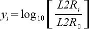
These three selections represent the L2 norm of the residual from each iteration of each equation.  The L2 norm is the sum of the squares at each point.  All residuals graphed on the line graph are divided by the initial value of the residual and plotted on a log scale.  The visual representation that is actually shown on the line graph is given by eqn. (2) for each of the three solution equations.  Thus the residual history graphs always start out at a value of 0.0.
  residuals
(2)
Therefore, each integer decrease in the residual levels represents an order of magnitude reduction in the residual.  For time dependent problems, the residual has limited meaning, but for steady problems the residual should generally decrease by moving in the negative direction.  Note that the large number of iterations often required to generate a solution means that residual plots can often take a large amount of time to calculate and re-draw.
    Finally, regardless of what is plotted, Gryphon automatically scales both the x and y axes to fit the plotted data.  The user may override this by selecting manual scale and typing in values for the extents of the graph window.  All four boxes must be populated to use the manual scale.
    The bottom contour and geometry window works similarly.  The first choice available to the user is a pair of radio buttons which allows the contour graph to plot the item selected in the 1st line graph above.  Whatever is selected there is what will be colored onto the geometry.  The "plot 1st item above" radio button is only available if the first item above is active and plotted versus x.  Otherwise, "do not plot contours" is selected.  The contours themselves will completely fill in the geometry domain.  Coloring is based on a HSB model, and so the colors are proportional to wavelength.  Red colors represent the high values while blue and purple colors represent the low values.
    Since a dense grid will often obscure the contour shading, it is often useful to turn off the grid lines for plotting.  Below the radio buttons are a series of check boxes.  The user may elect to remove the grid lines the area shape lines, or the physical model domain with the associated yellow highlighting.  These things may be turned back on at any time.  Usually, one is no longer interested in the physical model once a grid is created, so the physical model is automatically turned off when a new grid is created or imported.  This can be turned back on if it is necessary.  Grid lines and the area profile are plotted by default.
    Finally, the contour and geometry window can be manualy scaled at the bottom of its panel by selecting it and entering the domain range to plot.  Automatically scaling the window will always show the entire domain.  It is useful to note that if both graphing windows have autoscaling turned on, the x values will line up vertically between the graphs.  This makes for easy visual comparisons between the two windows.
    It is important to note that the solution consists of cell averages, which are assumed to be located at the cell centers -- not at the grid points.  The solution is plotted this way.  Further, with respect to the contour shading, each cell is uniformly shaded by its cell average.  Although an interpolation routine could have been used for shading between the cell centers, it was eventually decided to make the cells uniform as a specific reminder of the solution density.  Thus, a coarse grid solution will look coarse and remind the user that a denser solution may be needed.


<previous: Solution Options
up to Table of Contents
next: Solution Control >