Solution Management and Control

<previous: Graphing Options	up to Table of Contents	next: Evaluating the Solution >
open Reference Guide (in this window) open Applet Page (in new window)

Solution Management and Control

    A brief discussion must be made about managing solutions. A previous section discussed the application of initial conditions. There initial conditions are exactly what they claim to be. They are separate and distinct from any solution quantities stored. A concept which must be discussed is initialization of the grid. When a grid is first created, it is not initialized, which means that there is no solution information whatsoever associated with it. When the solve button is pressed in the Solution navigation panel, Gryphon first checks to see if the grid has been initialized yet. If not, it initializes the grid based on the specified initial conditions (believe it or not, there are default initial conditions if the user has done nothing so it is wise to check the initial conditions first). Once in an initialized state, the grid contains one solution level based on the initial conditions. In this way, the user can view the initial conditions exactly like any other solution data.
    The user can initialize the grid without solving anything by using the Solution submenu on the main window menu (Fig. 3c). Selecting "Initialize Grid" from this menu will initialize the grid using the initial conditions. If a solution is already present, the grid cannot be re-initialised without first removing it. This is done using the "Reset Solution" command. The user should be careful doing this and ANY and ALL solution data will be destroyed. Then, the user can re-initialize the grid using the "Initialize Grid" command. Unchecking the "continue existing solution" as discussed in the previous section has this same effect as selecting "Reset Solution" followed immediately by "Initialize Grid" before the solution proceeds. These commands can be useful if the solution is not stable and the user wishes to start over with better initial conditions or a lower CFL condition.
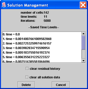
    A steady solution always have only one solution level. Each iteration erases the previous conditions. A transient problem, however, can have virtually unlimited numbers of solution levels. By default, the initial conditions are always saved, as are the final solution step data. And, of course, any multiple of the save frequency is saved. Since the user may wish to delete old time levels to save space, a more advanced solution management tool is available. It can be activated by selecting the "Manage Solutions..." command fro mthe Solution menu. The resulting dialog is shown in Fig. 19.

Figure 19. Detailed View of the Solution Management Dialog

At the top of the dialog is some basic statistics about the solution. The number of grid cells, the number of saved time levels, and the number of iterations in the history are all shown. Just below this is a list of all the available time levels listed in sequencial order by index number. The dimensional time is list at each index. The user may select one or multiple levels by holding down the CONTROL key and clicking on the time levels to remove. At the bottom of the dialog are two special options. The "clear residual history" checkbox will leave all solution data alone but delete all the iterations in the convergence history along with the three L2 norms of the residual of the equations. This is useful because several thousand residual values can take up a lot of storage space and tremendously slow down the visual graphing subroutines when redrawing the screen. Finally, at the bottom, the "clear all solution data" has the same effect as if the user selected "Reset Solution." This destroys all solution data and sets the grid to uninitialized status regardless of the selections in the rest of the dialog.
One final note is that the user can select to clear the residual history and select some time levels to delete at the same time. This is allowed. Pressing the "Delete" key performs the operation. The "Cancel" button makes no changes.

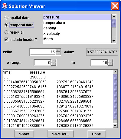
Figure 20. Detailed View of the Solution Viewer Dialog Box

    Visualization of a solution discussed separately in the previous section on graphing, but it is additionally appropriate to discuss the availability of looking at solution data in text form. Figure 20 shows the resulting dialog following the "List Solution..." command from the Solution menu. This dialog is meant for two purposes. First, it offers the user a quick look at the numbers of the solution, for verifying exact quantities, looking at feature details etc. Mostly, however, it is meant to allow the user to export data into a spreadsheet of graphing program. At the top left of the dialog box are the very same options that are available in the graph panels. The data available in each selection is the same, so the user should review Tables 1 and 2. The list window directly to the right changes to reflect the available options for each case. In this window the user can select one or many quantities to display by holding down the CONTROL key to select multiple quantities. Selecting a quantity again will disable it.
    Just below this box, the user may pick the constant spatial or temporal value associated with a listing, just as with the graphing windows. Listing temporal data for example will be done at whatever cell index is selected here. The same is true for spatial solutions at a given time level. The dimensional value of the x or t index is given just to the selector's right. Below this line is a range modifier. If one is looking for data at a particular location for example, it is not necessary to parse through a long list of numbers to find it. Grpyhon will show only the data within the range indicated. This applies to whatever data set is selected in the radio buttons at the top (spatial, temporal, or residual).
    Pressing the "Show" button will display the currently requested data in the text area. The checkbox near the top can be used to include or leave out a header line which lists the name of each quantity above its respective column. Whatever quantity is the selected independent variable will always be listed in the first column, followed by each dependent quantity in sequence, separated by tabs. The idea is that this text window can easily be used to copy and paste data into a spreadsheet program via the system clipboard. Alternately, pressing the "Save As..." button will allow the user to save the text area to a tab delimited text file. Pressing "Done" will close the dialog.

<previous: Graphing Options

up to Table of Contents

next: Evaluating the Solution >