Generating the Physical Model
Gryphon employs a very flexible 1-D model construction
and grid generation system. This system allows the user to create virtually
any distribution of grid points on the resulting computational model -- or
grid. The grid in Gryphon must consist of a set of pairs of points specifying
position and area at that position in the domain. Therefore, a physical
model must do several things. First, define the domain bounds. Second,
define the area profile in some way. Third, define the distribution of the
position of grid points throughout the domain.
Building a physical model in Gryphon starts with segments.
When the program is first initialized or the New command is selected
from the File menu, the generic physical model starts with one segment. There
must always be at least one segment; Gryphon will not allow this last segment
to be removed. The user can create more complex geometric representations
by adding segments to the model. Developing the physical model makes
heavy use of the Model navigation tab. This tab is shown in Fig. 5 for
reference throughout this section
Figure 5. Detailed
View of the Model navigation Tab
First, the domain can be simply defined in 1-D by two
points: the minimum x and the maximum x. These values can be input at
any time at the top of the model tab in the Domain panel. The values
show 0 to 1 as a default, but can be changed by selected the box and changing
the number. It is important to remember one thing: THE DOMAIN IS NOT
ACTUALLY CHANGED UNTIL ENTER IS PRESSED ON THE KEYBOARD. Fortunately,
Gryphon realizes that this may be forgotten sometimes, and higlights the box
bright yellow as soon as a change is made to either domain boundary. The
yellow border is removed when enter is pressed in the box. Then, the
change takes effect. The first or last segment respectively is automatically
extended or trimmed to conform to the new boundary. This is necessary
to correctly represent the domain, so it is usually better to define the
domain before inserting and manipulating a lot of segments. It just
makes things easier for the user.
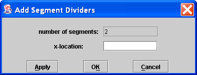
With the domain correctly bounded, one can begin managing
segments. One segment is always present at the start, but new segments
can be added by splitting the existing segment at a point, creating two child
segments. This is done in the Grid menu, with the Add Segment Divider
command. This opens the following dialog box shown in Fig. 6 which allows
one to type in a split point and split the segment. The total number
of segments present is shown, which updates every time one is split. The
segment spanning whatever x value is input is the one that is split to either
side of the split point. When the dialog is closed, the GUI contour
window is updated.
Figure 6. Detailed
View of the Add Segment Divider Dialog Box
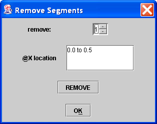
Likewise, it is possible to later remove segments using
the Delete Segment Divider option in the Grid menu. This dialog is shown
in Fig. 7, and removes the segment number indicated. The span of the
particuar segment in question is given just as a verification. When
the remove button is pressed, that segment is deleted from the physcial model
and the segment just after it is extended backward to fill the void. This
is true of all but the last segment, where the second to last segment becomes
the last segment and is extended to the domain end.
Figure 7. Detailed
View of the Delete Segment Dialog Box
The utility of dividing the domain into many segments
is that each individual segment can has its own area definition and grid point
distribution. This allows for very complex geometric and grid representations
to be created if the user wishes to take the time to do so. Once the
segments are laid out, it is time to generate area definitions. First,
the area definitions are created, and then attached to the segments one by
one. An area definition can be defined in two ways: (1) by specifying
an area rule, or (2) by importing a set of area points for an area table.
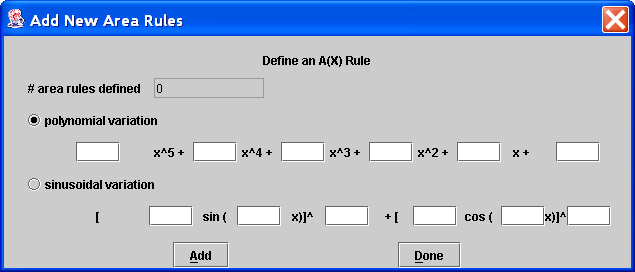
Area rules are simple. Selecting Add Area Rule
from the Grid menu opens the dialog box shown in Fig. 8.
Figure 8. Detailed
View of the Add Area Rule Dialog Box
In this dialog box, the user is inputting a formula for area as a function
of x. There are two choices, polynomial functions of up to 5th order,
or sinusoidal functions consisting of powers of sine and cosine. Either
option may be picked by the radio buttons. Then, each coefficient may
be typed in. All the coefficient boxes for the selected choice must
be populated, even if they are zero. Adding the area rule is accomplished
by pressing the "ADD" button.
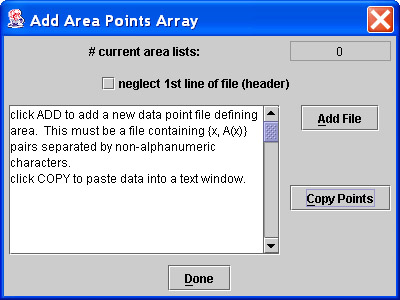
Alternately, the area may be defined discretely by specifying
a table of points from which to base an area definition. This involves
either importing a plain text file consisting of two columns of data separated
by tabs or spaces consisting of x - A(x) pairs or pasting data into a text
window from the system clipboard which conforms to the same standards. This
dialog box is shown in Fig. 9. This operation is very similar to importing
grid files in plain or copied text format from the File menu as discussed
in the previous section. That File option, however, creates a grid directly
point for point fro mthe file. This option can be useful if one has
previously made a more dense or less dense grid, for example, or one which
has a different density distribution. This way, the point distribution
can still be controlled.
Figure 9. Detailed
View of the Add Area List Dialog Box
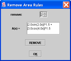
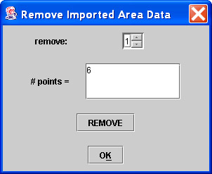
Either an area rule or an area list (table) can be deleted
if it is no longer needed in much the same way that a segment can be deleted.
Figure 10 shows these respective dialog boxes. In each case, information
about the area rule or list is given to make sure that the right one is being
deleted.
|
|
(a) Remove Area Rule
Dialog
|
(b) Remove Area List
Dialog
|
Figure 10. Detailed
View of the Remove Area Rule and Remove Area List Dialogs
Once the area distributions are defined, the last step
is to link the area distributions with the segments and define a point density
in each segment. This is accomplished easily in the Model navigation
tab, shown in Fig. 5. All the segments are kept numbered in spatial
order as they are added and deleted. Each segment is given a number
in sequence, and the active segment can be selected by using the spinner
at the top of the Segment panel in Fig. 5 which is labeled "segment #." The
active segment is highlighted in yellow on the contour window for further
clarification. Switching the spinner switched the active segment and
updates all its properties.
Associated with each segment is a number of grid divisions,
a division spacing, and an area definition. The grid divisions on each
segment can be changed in the box for that segment that is active. The
division spacing gives grid placement control. A spacing applied to
the active segment means that each successive cell will be a factor larger
than the previous cell. This factor must be larger than or equal to
1.0, and can be set up to apply in any of four directions: left-to-right,
right-to-left, center-to-edge, or edge-to-center. So, for example,
a division spacing of 2.0 left-to-right means that each element will be twice
as large as the one directly to its left. A center-to-edge spacing
of 2.0 will likewise mean that the single center element (if there is an
odd number), or two center elements (if there are an even number of divisions)
will be twice as large as those to either side. The ability to stagger
the grid placement in each segment coupled with the ability to subdivide
segments means that virtually ideal control is maintained over the grid topology.
Also, for all segment, either an area rule or an area list must be
applied to that segment. This can be chosen fro mthe radio buttons
and drop down boxes at the bottom of the segment panel. Pressing the
button labeled "VIEW" will display the currently selected area rule or area
list in a dialog box as a reminder of its properties.