Transonic Converging
/ Diverging Nozzle Tutorial
 Figure 21
. Transonic Nozzle Physical
Problem Definition
Figure 21 shows the nozzle geometry to be studied.
The domain of the nozzle runs from 0.0 to 1.0. The nozzle is
defined in three sections -- a straight section, a converging section, and
a diverging section. The respective area variations for these three
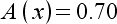
sections are given in Table 3.
Table 3. Area
Variation Polynomials by Zone for Transonic Nozzle
|
1
|
|
2
|

|
3
|

|
Inlet conditions are known completely in terms of Mach number, pressure,
and temperature. Two different cases will be studied with two different
outlet conditions. These boundaries will be discussed after creating
the geometry.
First, the physical domain needs to be divided to
reflect the three zones of the problem. This can be done by starting
Gryphon with a fresh physical model (the default when it starts up), and
switching to the model navigation tab (which is also the default). The
domain already runs from x=0.0 to x=1.0, so this can be left
alone. The default physical model initially starts with a single
segment within this domain. This can be changed by going to the Grid
< Add Segment Divider ... menu command at the top. In the simple
dialog that appears, enter a divider at x=0.25 and press "Apply" followed
by another divider at x=0.50 and press "OK". The tally in the
segment divider dialog should increase to 2 when the apply button is pressed.
After, the dialog clears, the GUI should update and the model should
look like the one shown in Fig. 22. This corresponds to the three
sections above in Fig. 21.
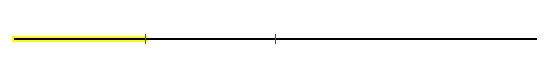 Figure 22
. Physical Model Domain
for Nozzle
Next, the areas need to be defined as given in Table
3. This is done by opening the algebraic area rule dialog from the
Grid < Add Area Rule... command. The three area rules can
be added in any order by selecting the polynomial variation in this dialog
and entering the coefficients in front of each polynomial term. After
each, press "Add." Press "Done" when finished. The number of rules
defined should increase after each is added. The final area rule is
shown in Fig. 23 after the "Add" button has been pressed (the tally shows
3 rules already present).
 Figure 23
. Area Rule Addition Dialog
After closing the area rule dialog, the area rules must
be attached to the segments and the number of divisions set for each segment.
Back in the model navigation tab, the segments can be indexed through
using the segment number spinner on that navigation tab. The currently
selected segment is highlighted in the graph window in yellow. The
radio button should be selected for using an area rule (rather than an area
list) by default in each segment, so the one needs only to select the appropriate
area 1 - 3 for each. While doing this, set the number of divisions
to 12 for segment 1, 24 for segment 2, and 75 for segment three, with spacing
ratios of 1.02 left-to-right, 1.065 right-to-left, and 1.01 left-to-right
for segments 1 to 3 respectively. These values are summarized in Table
4.
Table 4. Grid
Related Parameters for Transonic Nozzle Cases
|
segment #
|
area rule
|
divisions
|
spacing
|
space orientation
|
1
|
1
|
12
|
1.020
|
left-to-right
|
2
|
2
|
24
|
1.065
|
right-to-left
|
3
|
3
|
75
|
1.010
|
left-to-right
|
Figure 24 shows what the model navigation bar should look like for the
second segment as an example.
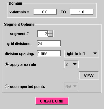 Figure 24
. Model Navigation Tab Showing
Segment #2 Parameters
After setting this up, press "Create Grid" and the grid
should be automatically generated. This result is shown in Fig. 25.
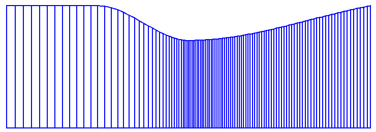 Figure 25
. Transonic Nozzle Grid
Now is a good time to save the model information. If
the program is not being run as an applet in protected mode, one may go
to the file menu and select File < Save.... This will bring
up a dialog, and a suitable name can be entered. Enter something like
"nozzle" in the space provided. Gryphon automatically appends a ".egd"
extension to the database.
Next, move to the BC navigation tab, and enter the boundary
condition information. The inlet should be applied at the left boundary.
Gryphon should have defaulted to an inlet condition here already.
Since the inlet boundary is to be a steady (constant) boundary, the
inlet conditions can be set by pressing the "modify" button. Select
"pressure, temperature" from the property selection box, and enter inlet
conditions of 250,000 for pressure and 350 for temperature. Select
"Mach" and enter 0.450 for a Mach number. The dialog may then be closed
by pressing the "OK" button.
Case #1: Extrapolated Nozzle
Two separate outlet boundaries will be studied. The
first case is for a constant extrapolation boundary on the outlet. This
is Gryphon's default for the right boundary, so this information may be
left alone. For initial conditions, the default of initializing via
the left boundary is a good choice for this problem.
The solution options for this problem may be set in
the solution navigation tab. The summary of the options is shown in
Fig. 26, which shows the solution tab as it should be configured.
 Figure 26
. Solution Navigation Tab
The problem is steady-state, and the number of iterations should be set
to 5,000. This is sufficient to fully converge this case, a fact which
shall be shown to be true shortly. The Euler Implicit scheme should
be selected as the time integration scheme. Set the CFL condition
to a localized limit, and enter a value of 1.0. This is a higher value
than can be used for an explicit scheme, but this value is a good choice
for implicit methods. The default of 3rd order is fine for the MUSCL
interpolation technique, but the limiter shoudl be changed to the van Albada
limiter. The limiter should not be particularly active for this case
since its solution will involve no shocks, but the min-mod limiter can affect
convergence during the transient start-up of the problem. Select the
Roe scheme as the flux scheme to be used since it offers the greatest accuracy.
Pressing the "SOLVE" button starts the solution. Gryphon
will show the solver dialog listing the progress in the solution. The
entire 5,000 iterations should typically take on the order of 1 - 2 minutes
to complete, but may vary significantly depending on the processor architecture
and operating system available. During this solution process, the
graphing window will show a real-time progress of the residual levels. The
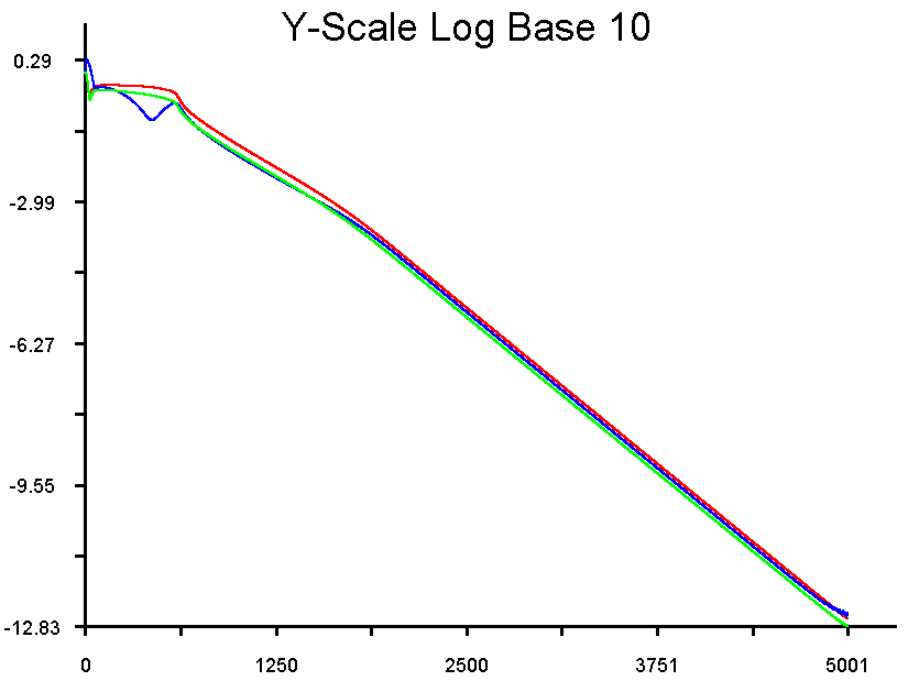
result of this residual monitoring is shown in Fig. 27.
Figure 27. Residual
History for Case #1: Outlet Extrapolation
This is the indication that excellent convergence is achieved by the end
of 5,000 iterations. The residual levels have dropped approximately
12 orders of magnitude and are close to machine zero.
With the solution available, it is again a good time
to save the newly generated data. Selecting File < Save...
from the main menu will do this. The solution data is included in the
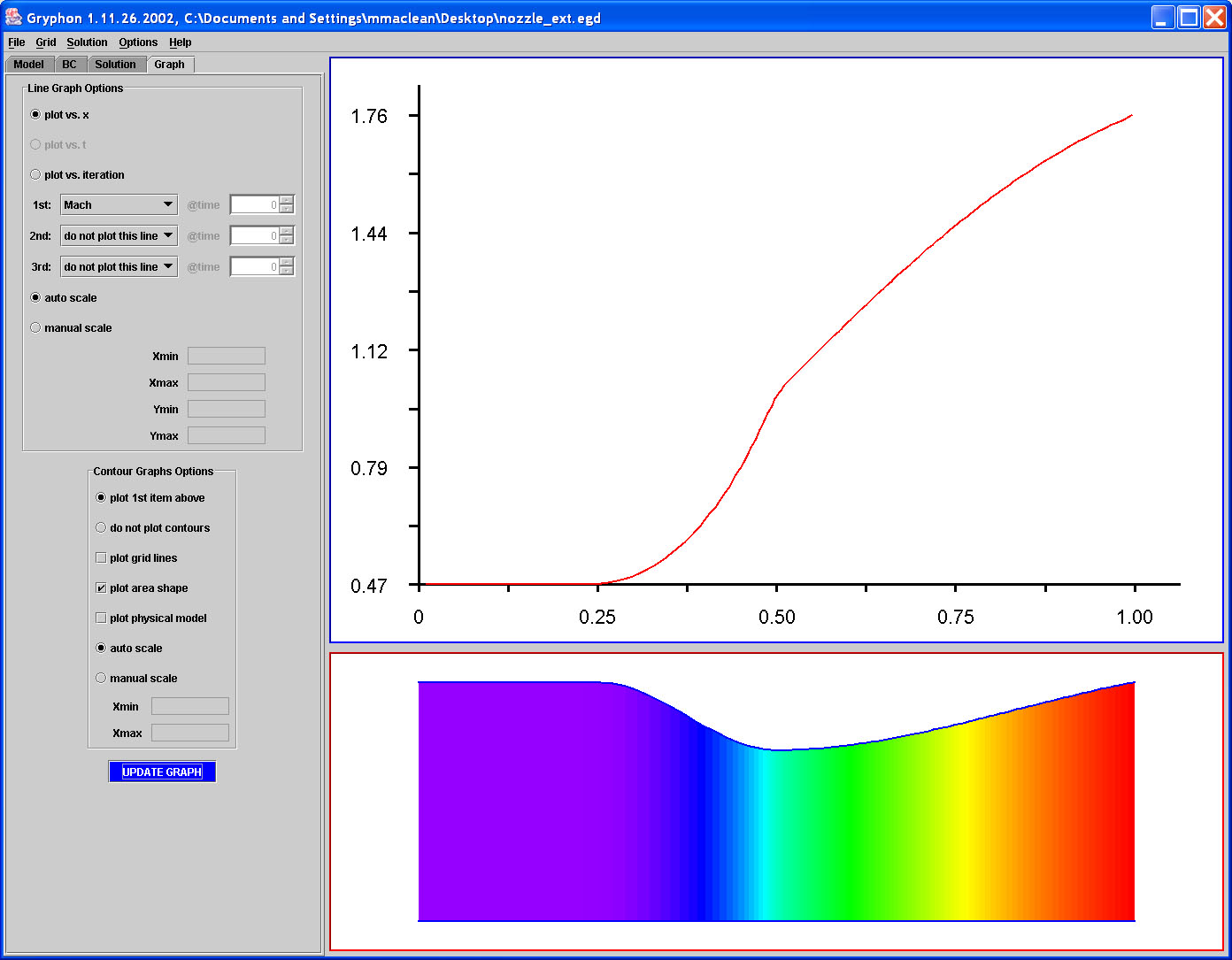
latest save. It is then possible to look at the solution by going to
the Graph navigation tab. Here, select at the top in the line graph
panel to "plot versus x" by selecting the proper radio button. From
the line labeled "1st," select Mach number from the pull-down menu. Then,
at the bottom under the Contour Graph Options panel, choose to plot the first
item above by selecting the radio button labeled so. It is also helpful
to uncheck the box labeled for the grid lines. Press the "Update Graph"
button, and the graph of Mach number should be shown in the upper window
and the Mach number distribution should be shaded on the geometry in the
lower window. This scene is shown in Fig. 28.
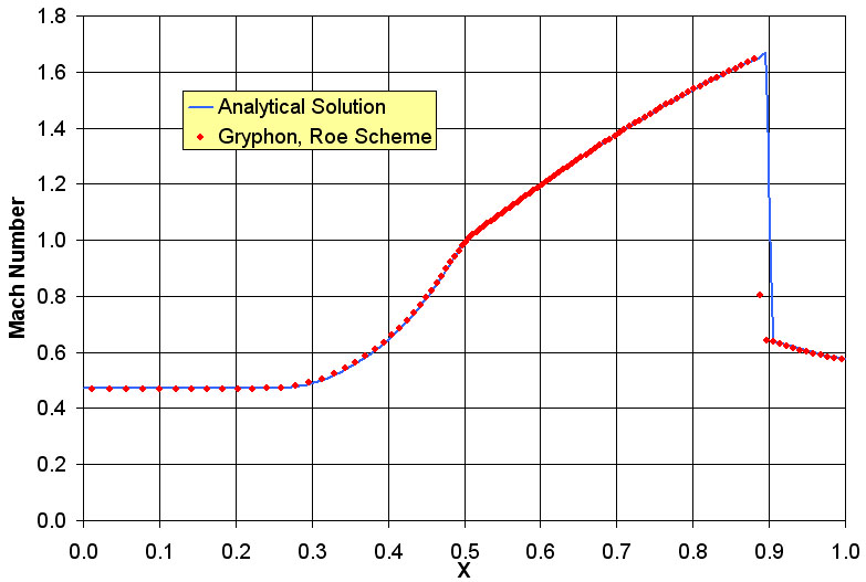
This solution can be compared with the expected solution
for validation purposes. From Anderson [1993],
the solution for a shockless nozzle with a supersonic outlet condition can
easily be found using the principles of inviscid quasi 1-D flow. The
prediction is accurate almost to the point of perfection throughout the
domain. The comparison between the analytical prediction and the Gryphon
solution is shown for the Mach number in Fig. 29. Also, it is worthwhile
to notice that the Mach number does indeed equal 1.0 at the throat as it
should.
Figure 29. Mach Number
Comparison between Analytical and Gryphon Solutions for Case #1: Outlet
Extrapolation
Case #2: Nozzle with Back Pressure
The second case which will be studied is that of a nozzle
with a known back pressure.This case is different and more complex than
the first case in that a subsonic outflow will be created by selection of
the back pressure strength and a shock will form in the nozzle. The
back pressure can be set by going back to the BC navigation tab. Here,
change the right boundary selection to "back pressure / subsonic out." Then,
press the "modify" button for this boundary and enter a value of 200,000
in the text box provided. This sets a back pressure of 80% of the inlet
total pressure.
The solution needs to be reset to run this case properly.
This also affords the opportunity to test a few of Gryphons other
features. By opening up the Solution menu, and selecting the Solution
< Reset Solution command. Gryphon will display a warning message
saying that the solution data will be deleted. This is fine. Then,
re-initialize the data by selecting the Solution < Initialize Grid
command. Since the initial conditions are specified to come from the
left inlet boundary, the entire flowfield should now be set to the subsonic
inlet conditions.
Since this problem is slightly more complex, a similar
level of convergence to case #1 requires that 7,500 iterations be used,
so the iterations should be changed to this on the Solution navigation panel.
Before solving, it is wise to save the model again, so this time,
select File < Save As... from the file menu at the top and enter
a new name for the model to avoid overwriting the other case. A name
like "nozzle_shock" is fitting, and Gryphon will again append the proper
extension to the name. Once saved, the solution can be generated by
pressing the "SOLVE" button. The residual history is similar to the
first case. It looks like that shown in Fig. 30.
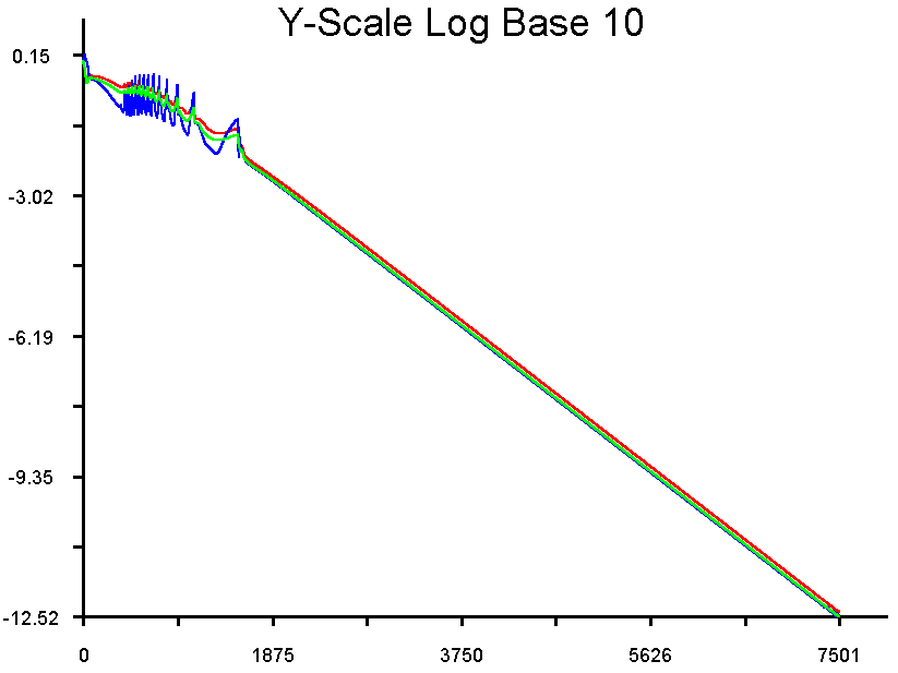 Figure 30
. Residual History for Case
#2: Specified Back Pressure
The resulting Mach number distribution for this case is shown in Fig. 31.
This plot is produced by following the instruction given at the end
of the first case above.
Finally, Fig. 32 shows a comparison of Mach number and pressure distribution
with analytical prediction methods for this case. For an analytical
prediction, invscid equations had to be connected to the analytical equations
for a normal shock. This requires an iterative process to properly locate
the shock. As such, the analytical solution is also somewhat approximate.
However, the agreement between the two solutions is evident.
(a) Mach Number Comparison

(b) Pressure Comparison
Figure 31. Comparison between Analytical
and Gryphon Solutions for Case #2: Specified Back Pressure
One should notice in particular that the pressure does actually go to 200,000
at the outlet as the boundary condition specified.
<previous:
|
up to Tutorials
|
next: Shocktube Tutorial >
|